Fitting an SNN to do a Classification Task

In the example below, we will use gradient descent to fit the parameters of an SNN. Since Jaxley implements surrogate gradients for Fire channels by default, we can backpropagate through the entire network, despite the SNN implementing non-differentiable functions.

import jax
import jax.numpy as jnp
import matplotlib.pyplot as plt
import optax
from jax import config
from tqdm import tqdm

import jaxley as jx
from jaxley.channels import Fire, Leak
from jaxley.synapses import SpikeSynapse

# Set up configuration
config.update("jax_enable_x64", True)

dt = 1e-3
T = 0.20

reset_voltage = 0.0
tau_mem = 10e-3

# Define the initial parameters of the channels
params_init_Leak = {
    "Leak_gLeak": jnp.array(tau_mem),
    "Leak_eLeak": jnp.array(reset_voltage),
}

params_init_Fire = {
    "Fire_vth": jnp.array(1.0),
    "Fire_vreset": jnp.array(reset_voltage),
}

Simulation and network hyperparameters

Set RNG seed, sizes of each layer, and build the network (input → hidden → output). Note that the output neurons are created without Fire channels because we will read their membrane potentials rather than their spikes for classification.

# Set seed and layer sizes
seed = 1701
key = jax.random.key(seed)
batch_size = 256
n_input = 100
n_hidden = 4
n_output = 2

# Create network
neurons = [jx.Compartment() for _ in range(n_input + n_hidden + n_output)]
net = jx.Network(neurons)

# Set the parameters of the neurons
net.select(nodes="all").insert(Leak())
net.select(nodes=range(n_input + n_hidden)).insert(Fire())
for param in params_init_Leak.keys():
    net.select(nodes="all").set(param, params_init_Leak[param])
for param in params_init_Fire.keys():
    net.select(nodes=range(n_input + n_hidden)).set(param, params_init_Fire[param])
net.select(nodes="all").set("length", 1.0 / (2 * jnp.pi * 1e-5))
net.select(nodes="all").set("radius", 1.0)  # 1.0 is also the default.
net.select(nodes="all").set("v", 0.0)

# index ranges of layers in network
hidden_end = n_input + n_hidden
output_end = hidden_end + n_output
input_range = range(n_input)
hidden_range = range(n_input, hidden_end)
output_range = range(hidden_end, output_end)

# connect neurons
jx.fully_connect(net.cell(input_range), net.cell(hidden_range), SpikeSynapse())
jx.fully_connect(net.cell(hidden_range), net.cell(output_range), SpikeSynapse())


def normal(subkey, mean, std, shape):
    return mean + (jax.random.normal(subkey, shape) * std)


# Set random synaptic weights
parameters = None
l1_edges = n_input * n_hidden
l2_edges = n_hidden * n_output
key, subkey = jax.random.split(key)
gs_l1 = normal(subkey, 0.0, 10.0, (l1_edges))
gs_l1 = [{"SpikeSynapse_gS": gs_l1}]
key, subkey = jax.random.split(key)
gs_l2 = normal(subkey, 0.0, 10.0, (l2_edges))
gs_l2 = [{"SpikeSynapse_gS": gs_l2}]

for edge in range(l1_edges):
    net.select(edges=edge).set("SpikeSynapse_gS", gs_l1[0]["SpikeSynapse_gS"][edge])

for edge in range(l2_edges):
    net.select(edges=(l1_edges + edge)).set(
        "SpikeSynapse_gS", gs_l2[0]["SpikeSynapse_gS"][edge]
    )

net.select(edges="all").make_trainable("SpikeSynapse_gS")

parameters = net.get_parameters()

Number of newly added trainable parameters: 408. Total number of trainable parameters: 408

Creating input currents / dataset

For this toy classification task we sample Poisson spike trains for the inputs and convolve them with a small kernel (i_min) to create continuous input currents. We then pack batch_size such examples into current_batches which will be used for training.

i_min = jnp.array([508.0] * 2)
freq = 5  # Hz
prob = freq * dt
key, subkey = jax.random.split(key)
mask = jax.random.uniform(subkey, (batch_size, n_input, int(T / dt)))
x_data = jnp.where(mask < prob, 1.0, 0.0)

current_batches = jnp.array(
    [
        [jnp.convolve(i_min, x_data[i][j], "same") for j in range(n_input)]
        for i in range(batch_size)
    ]
)

net.delete_recordings()
net.cell(output_range).record("v")

Added 2 recordings. See `.recordings` for details.

Simulation helpers

simulate_network runs a single simulation and returns the voltage traces of the output neurons. We JIT-compile and vectorize over batches with simulate_network_batches so training is faster.

def simulate_network(params, current):
    """Simulates the network, returning the voltage traces of the output neurons"""
    data_stimuli = net.cell(range(n_input)).data_stimulate(current, None)
    return jx.integrate(
        net,
        data_stimuli=data_stimuli,
        params=params,
        delta_t=dt,
        t_max=T,
    )


simulate_network_batches = jax.jit(jax.vmap(simulate_network, in_axes=(None, 0)))

Loss and accuracy

We compute the maximum membrane potential across time for each output neuron and apply a softmax to those maxima to obtain class log-probabilities. The loss is the standard cross-entropy between the predicted log-probabilities and one-hot targets. The get_accuracy helper computes a simple classification accuracy using argmax of the maxima.

def cross_entropy(logprobs, targets):
    target_class = targets
    nll = jnp.take_along_axis(logprobs, jnp.expand_dims(target_class, axis=1), axis=1)
    ce = -jnp.mean(nll)
    return ce


def loss_fn(params, targets):
    voltages = simulate_network_batches(params, current_batches)
    maximums = jnp.max(voltages, axis=2)
    log_p_y = jax.nn.log_softmax(maximums, axis=1)
    return cross_entropy(log_p_y, targets)


key, subkey = jax.random.split(key)
targets = jnp.where(
    jax.random.uniform(subkey, (batch_size), minval=0.0, maxval=1.0) < 0.5, 1, 0
)


def get_accuracy(params):
    voltages = simulate_network_batches(params, current_batches)
    maximums = jnp.max(voltages, axis=2)
    am = jnp.argmax(maximums, axis=1)  # argmax over output units
    acc = jnp.mean((targets == am))  # compare to labels
    return acc

Optimization and training

We use optax.adam to optimize the synaptic weights (which we flagged as trainable earlier). The training loop JIT-compiles the gradient computation and updates the parameters on each epoch. We also display a progress bar using tqdm with the current loss and accuracy.

grad_fn = jax.jit(jax.value_and_grad(loss_fn, argnums=0))
optimizer = optax.adam(learning_rate=0.1)
opt_params = parameters
opt_state = optimizer.init(opt_params)

n_epochs = 500
with tqdm(total=n_epochs, desc="Training") as pbar:
    for epoch in range(n_epochs):
        loss, gradient = grad_fn(opt_params, targets)

        # Optimizer step.
        updates, opt_state = optimizer.update(gradient, opt_state)
        opt_params = optax.apply_updates(opt_params, updates)
        pbar.set_postfix(
            {"Loss": f"{loss:.4f}", "Accuracy": f"{get_accuracy(opt_params):.3f}"}
        )
        pbar.update()

Training: 100%|████████████████████████| 500/500 [12:19<00:00,  1.48s/it, Loss=0.2618, Accuracy=0.883]

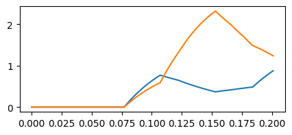
Visualizing output voltages

Finally, we run a simulation with the learned parameters and plot the output membrane potentials across time. Since output neurons don’t fire in this example (we never inserted Fire channles into them), we inspect their voltages directly to decide the predicted class. The predicted class is determined by the neuron’s maximum voltage.

v = simulate_network(opt_params, current_batches[0])

time_vec = jnp.arange(0, T + 2 * dt, dt)
fig, ax = plt.subplots(1, 1, figsize=(5, 2))
_ = plt.plot(time_vec, v.T)
plt.show()